- A risk parity strategy could be applied to fixed-income-only portfolio, and potentially still achieve a higher risk-adjusted return than a benchmark.
- We believe portfolio constraints, the asset universe selection, lookback period and rebalance frequency are key variables that determine the performance of a risk parity portfolio.
- The maximum drawdown of our hypothetical risk parity portfolio was smaller during modest market downturns, but was greater during market crises, a trait that is related to the selected asset universe and lookback periods of the simulation.
- Our simulation showed a leveraged risk parity portfolio could potentially achieve a higher total rate of return than a fixed-income benchmark with the same quantity of risk. Leverage, however, can also magnify losses when used in a risk parity portfolio.
Introduction
A risk parity strategy is an asset allocation strategy that can be used for both strategic and tactical asset allocation. It aims to achieve better diversified portfolios by balancing the risk contribution of various asset classes. The strategy uses asset beta/covariance and does not require return assumptions for the asset classes being utilized. The strategy also can be used for risk budgeting and factor tilting, once the base model has been established. One advantage of applying a risk parity strategy is that the model can be rebalanced mechanically based on an algorithm, which can reduce human error emanating from decisions and judgements made during times of higher emotion and stress. Care needs to be taken not to change a chosen algorithm during times of higher emotion or stress as that process negates the objective of reducing human/judgmental impacts on this investment strategy approach.
The key concept of a risk parity strategy can be mathematically represented by the following formula1. The risk contribution from each asset to the overall portfolio total risk is the same.
𝑥i and 𝜕xi represent the weight and beta of the 𝑖th asset respectively; 𝑥j and 𝜕xj represent the weight and beta of the 𝑗th asset. The weight of each asset, 𝑥, is between 0 and 1. The sum of 𝑛 asset weights equals to 100%. 𝜕xi𝜎(𝑥) is marginal risk contribution of the 𝑖th asset.

Risk parity strategies have become increasingly popular and familiar to institutional investors over the past few decades2. In this study, we explore the feasibility of applying the strategy to fixed-income-only portfolio, which may be more interesting to insurance asset and pension fund managers. The effectiveness, implementation variables and limitations of this strategy when applied to a fixed-income-only portfolio are the focus of this report.
Data
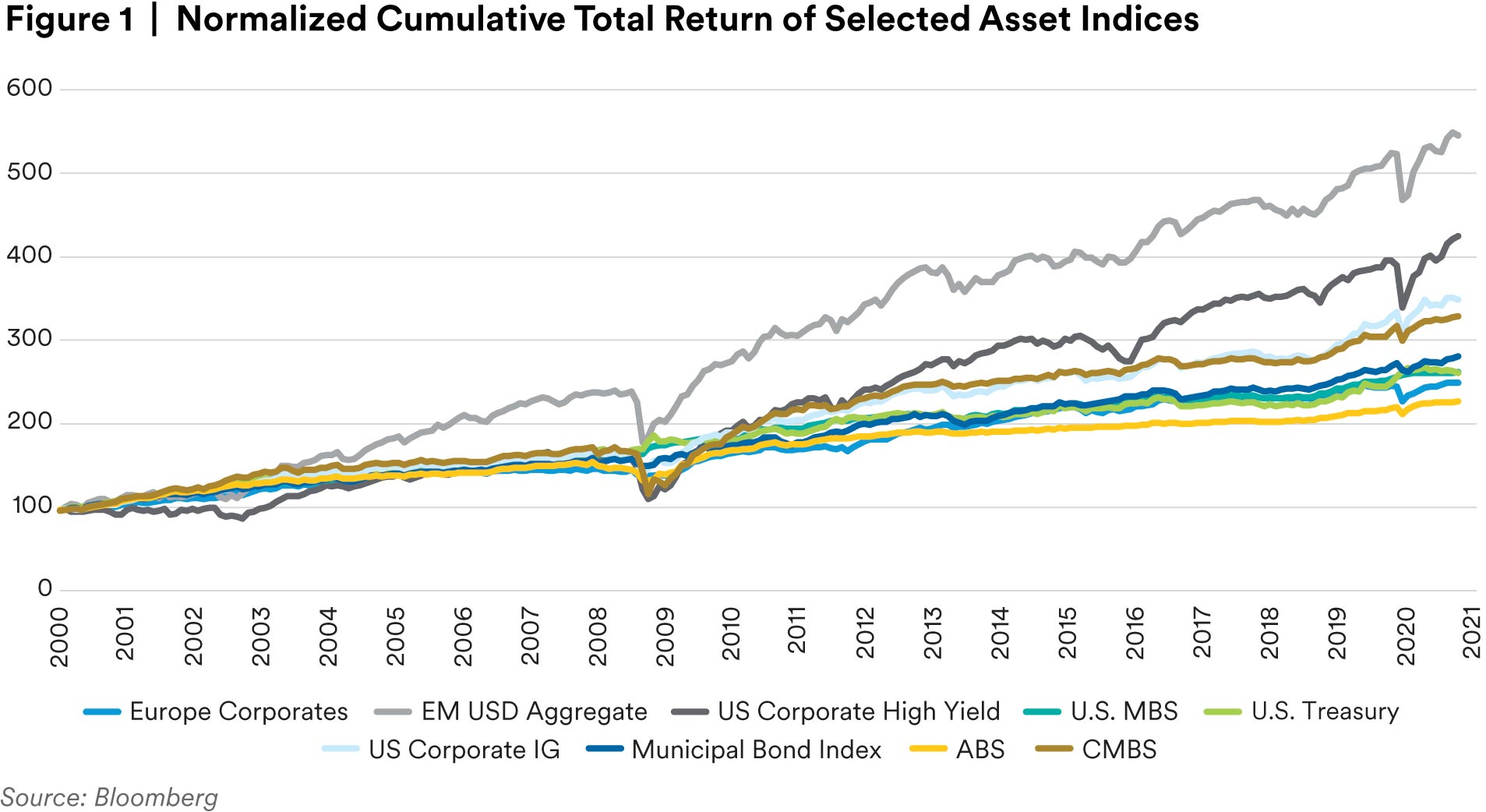
As shown in Table 1, we used nine asset indices that were selected to represent major public fixed income sectors, taking into account both the data availability and the available history. The Bloomberg Barclays Global Aggregated Total Return Index (“Global Agg Index”) was used as the benchmark. There are several sectors in the Global Agg Index that are not included in the selected asset universe and vice versa. For the assets that are included in both, the weights of these assets in the risk parity portfolio could be significantly different from those in the Global Agg Index. Therefore, the Global Agg Index should only be viewed as an overall fixed income market gauge, rather than a strict benchmark. Some of the selected assets are highly correlated. Adding lower- and negatively- correlated assets (such as private corporates and commercial mortgages) might further improve portfolio performance and risk profile. However, adding these more risky and illiquid assets would introduce rebalancing constraints, because of the trading cost and risk-based capital requirements, which are portfolio specific. Therefore, to generalize the findings of this report, only pubic indices were selected, and no criteria of asset correlation was applied for selecting these assets.

Extremely low volatility assets were also not included, e.g., cash and short term, since these extremely low volatile assets would be assigned an extremely high weight when applying a risk parity strategy. Therefore, portfolio returns would be very low, although relatively more stable. Both weekly and monthly data were used. Figure 1 shows the cumulative returns of the selected asset indices. All indices were normalized at 01/01/2000.
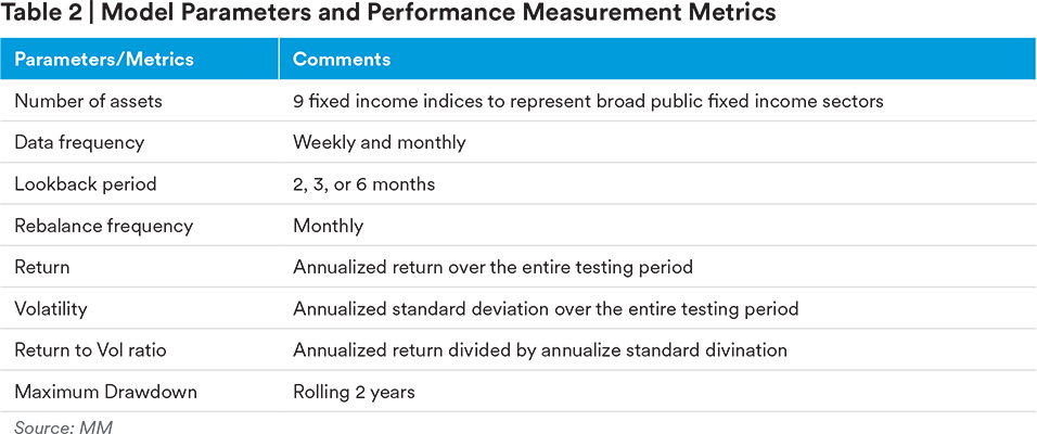
Model Parameters and Metrics
Rebalance was done at a monthly frequency. The rebalancing objective was to achieve an equal risk contribution from each asset by finding the appropriate weight combination. To calculate asset standard deviation and the covariance matrix, the lookback period and data frequency need to bedetermined. From our hypothetical back-testing results in the next section we found that these two were the most important variables, providing that the asset universe had been defined. For performance measurement, higher return does not necessarily mean that the strategy is better, because the associated risk needs to be considered. Therefore, a return-to-volatility ratio, a risk adjusted risk measure, was used to evaluate portfolio performance. The higher the return-to-volatility ratio, the better the portfolio performance. Maximum Drawdown (MDD) was used to measure the portfolio risk profile. A 2-year rolling window was used for MDD.
Results and Discussion
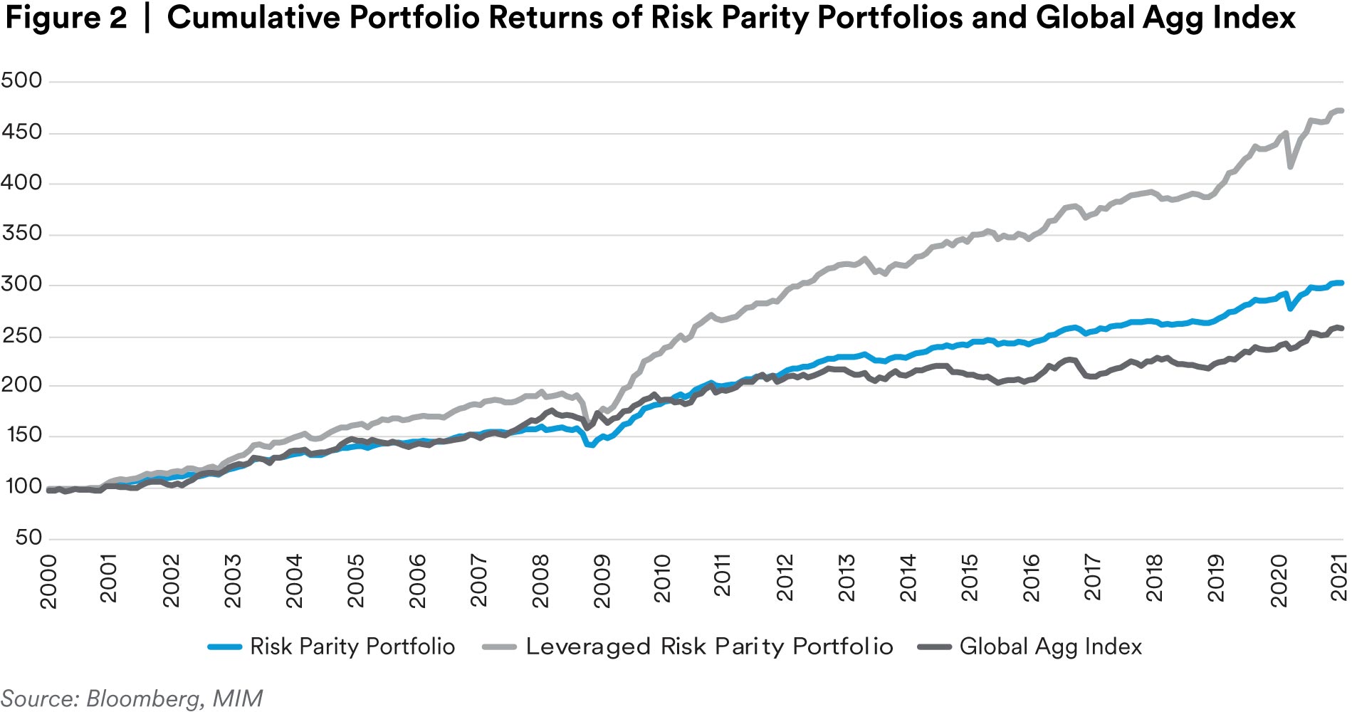
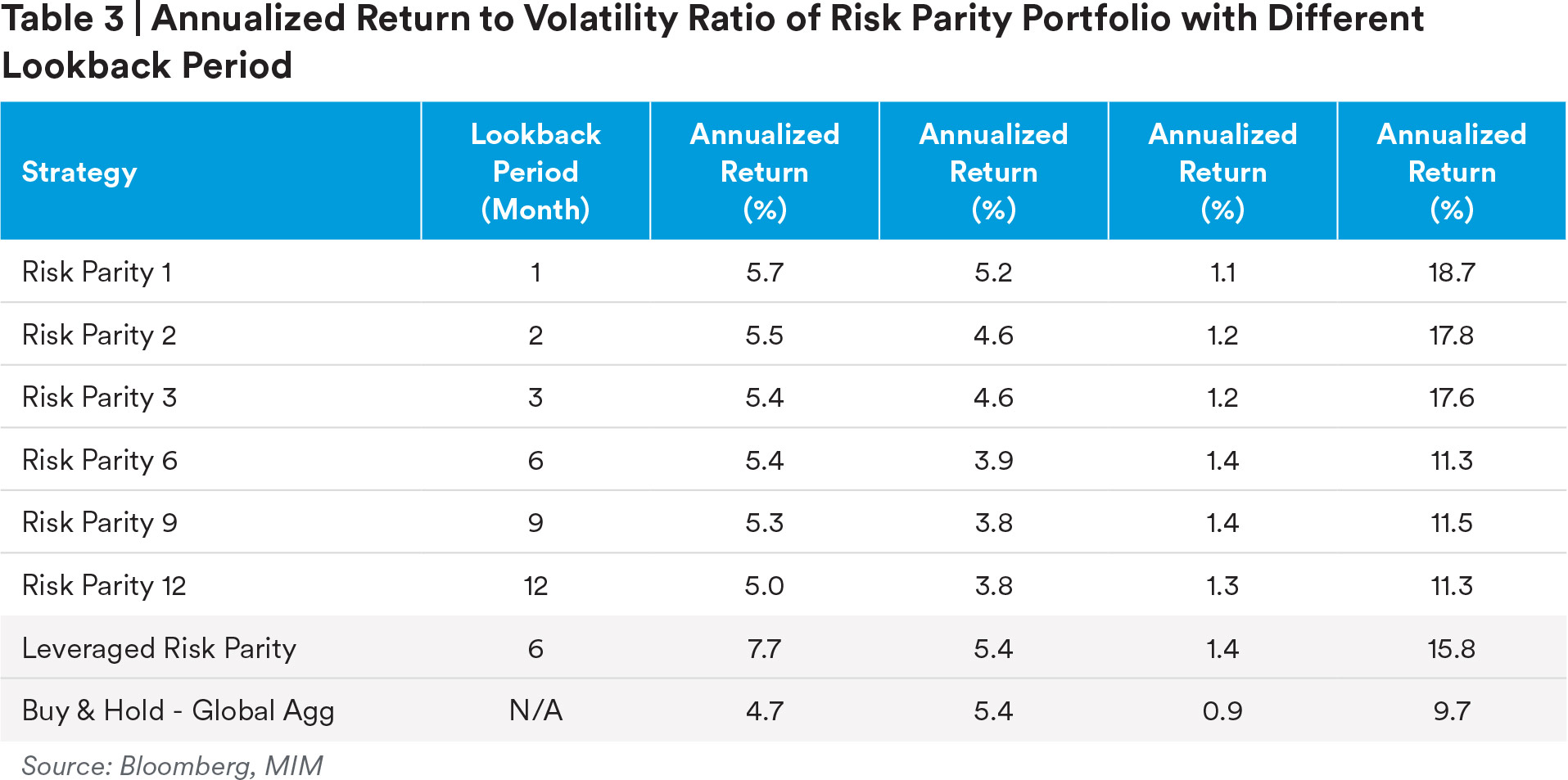
Figure 2 shows that in our simulations the risk parity portfolio with 6-month lookback period (the blue line) produced not only a higher cumulative return but also a higher return-to-volatility ratio than those of the Global Agg Index (the dark gray line). Several lookback periods were tested (ass hown in Table 3). The first observation is that, the risk parity portfolios with different lookback periods all outperformed the Global Agg Index, a buy and hold strategy. This shows that the hypothetical risk parity portfolio achieved a higher risk-adjusted return, with robustness, over the periods tested. Second, as the lookback period increases, both annualized return and annualized volatility decreased. However, the return-to-volatility ratio reached its highest level of 1.4 with 6- and 9- month lookback periods. The ratio diminished when the lookback period was increased to 12-months. Since the assets with relatively higher volatility will be underweighted, especially when overall market is in a downturn, the hypothetical risk parity strategy effectively scaled down the portfolio’s risk exposures and improved the performance over time periods tested. If the lookback period is too long, the portfolio may not be sensitive enough to adapt to the changes in market volatility. On the other hand, if the lookback period is too short, the strategy is too sensitive to asset volatility changes and produces asset allocation shifts too frequently, which creates a lot of “whipsaw” trades and causes underperformance. Our back-testing results support this explanation. We believe that 6- to 9- months is a reasonable lookback range that achieves a balance between the under- and over-reaction for the selected asset universe.
In this report, the lookback period was not optimized for two reasons. First, the optimization in back-testing could introduce a data-mining issue. Second, the optimal lookback period is specific to the selected asset universe, data frequency and benchmark. When the asset universe and other constraints change, the optimal lookback period may change accordingly. Our goal is to explore and demonstrate the implementation factors and evaluate the applicability of risk parity strategy in a fixed-income-only portfolio, rather than providing a specific strategy with a defined universe and a set of parameters.
The hypothetical risk parity strategy with a 6-month lookback period was chosen to demonstrate the frequency and magnitude of the asset weight changes overtime, as shown in Figure 3. As can be seen, the riskier assts, e.g., US Corporate High Yield, were underweighted in the model when the sector volatility increased during the 2008 financial crisis and other market downturns. The shorter the lookback periods and the higher the rebalance frequency, the more frequently the asset weights shift. Besides the whipsaw effects, frequent weight changes also increase transaction costs, given the nature of fixed income securities and illiquidity assets, if included. For simplicity reasons, transaction costs and other portfolio fees and expenses are not considered in the back-testing results herein. Transaction costs and fees and expenses will reduce performance when a strategy is implemented. Regardless how frequently the asset weights changes, the risk contribution from each asset remains the same, as shown in Figure 4, which is the definition of risk parity strategy.
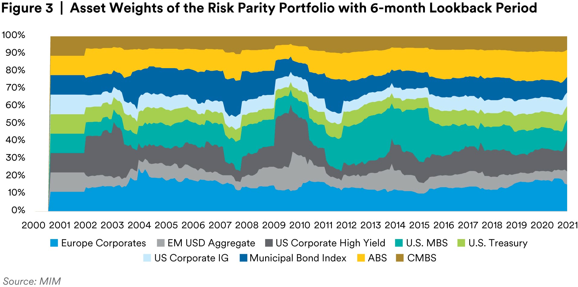
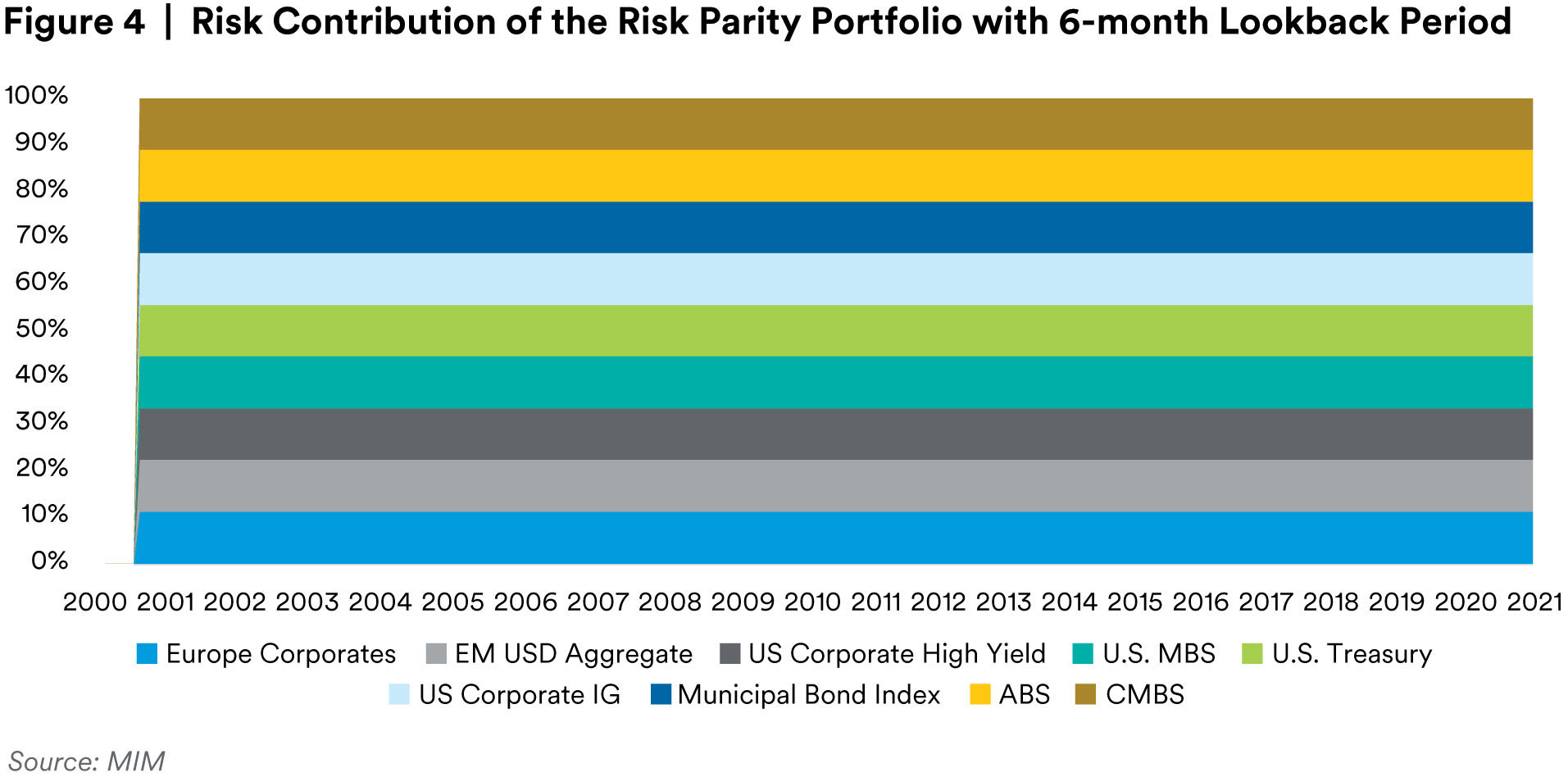
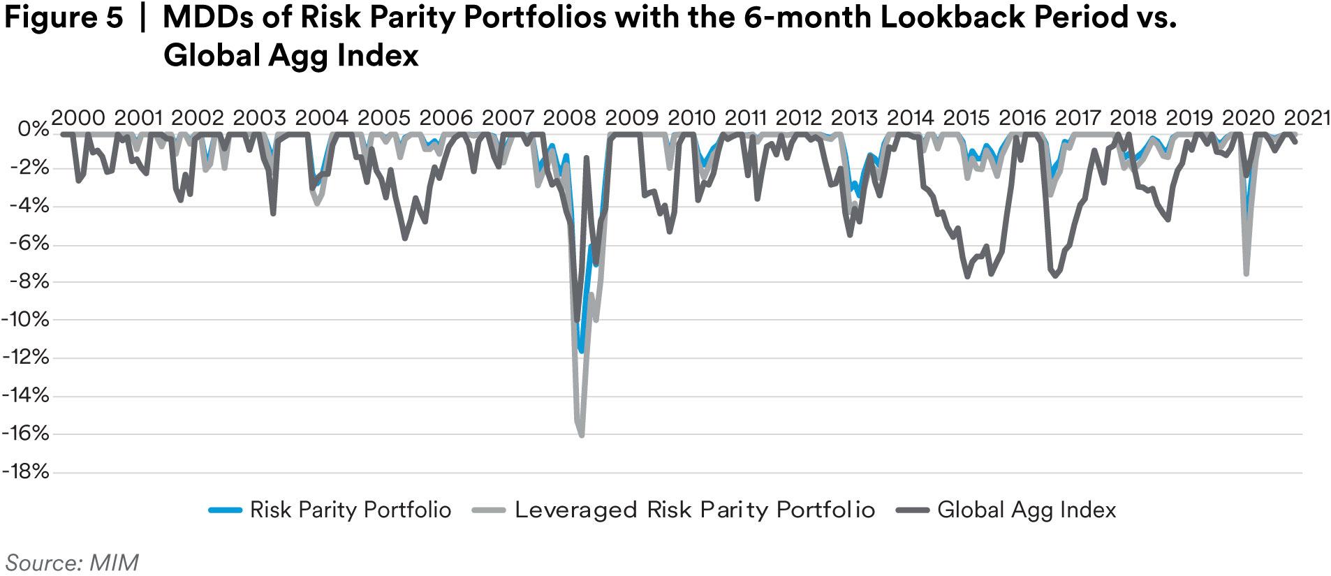
Figure 5 shows that the risk parity portfolio had a smaller Maximum Drawdown (MDD) than the Global Agg Index in most of the testing periods from 01/01/2000 to present. However, the MDDs of the risk parity portfolio were larger during the 2008 Great Financial Crisis and during the current pandemic (March 2020). The combination of the asset universe, rebalance frequency and lookback periods determined the portfolio risk profile in terms of MDD. The risk parity portfolio included riskier assets, such as High Yield and CMBS. During crises, the values of these riskier assets dropped suddenly. The monthly rebalance frequency was not able to cut down the weights of these asset quickly enough, therefore, the MDDs of the risk parity portfolio were bigger than those of Global Agg Index during crisis periods. In a relatively slow-moving bearish market, the risk parity portfolio with a 6-month lookback period and monthly rebalance frequency was able to adjust the weights more gradually. Therefore, the MDDs of the risk parity portfolio were smaller than those of the Global Agg Index during a slow-moving market.
Although our simulation suggests a risk parity strategy could potentially achieve a higher risk adjust return, it is not necessarily the case that the total return is always higher than that of a benchmark. The main reason could be that the risk parity portfolio is not taking enough risk, so the total return of the risk parity portfolio underperforms the benchmark in terms of total return. In order to try and boost the total return, leverage could be used to adjust the overall portfolio volatility to the benchmark level. Two common leverage methods are borrowing cash and using derivatives (e.g., total return swaps). Borrowing costs and collateral requirements need to be considered respectively for the two methods. It should be noted, however, that while leverage can be used in an effort to boost total return, leverage can also magnify losses that would not occur in the absence of leverage.
In Figure 2, the light gray line shows that in our simulations the leveraged risk parity portfolio significantly outperformed the Global Agg Index, while maintaining the same amount of risk (i.e., volatility) as the Global Agg Index and the same return-to-volatility ratio as the unleveraged risk parity portfolio (see Table 3). The leveraged portfolio returns were calculated by multiplying the return-to-volatility ratio (1.4) of “Risk Parity 6” portfolio by the volatility (5.4%) of the Global Agg Index. No specific leverage method was modeled in this leveraged portfolio. The MDD of the leveraged risk parity portfolio was bigger than that of the unleveraged portfolio during crisis periods, as shown Figure 5. Leverage cost was not considered in the leveraged risk parity strategy, since the leverage cost could be different for each firm. Nevertheless, we believe these costswould not eliminate the outperformance of the strategy in our simulation.
Summary
The back-testing results showed that a hypothetical risk parity strategy could be applied to a fixed-income-only portfolio and achieve a higher risk-adjusted-return than that of a fixed income benchmark. Our simulation indicated that the asset universe selection, lookback period for volatility/covariance calculations and rebalancing frequency were the key variables for successfully implementing the risk parity strategy described. The risk target and tolerance, in terms of volatility and maximum drawdown, define the portfolio’s risk profile. Leverage can also be a useful tool to try and boost the total return of a risk parity portfolio, while maintaining the same amount of risk as the benchmark, or at any desired risk level.
Future work
Adding constraints, such as volatility and risk-based capital, could help adjust the risk profile of risk parity portfolio, in order to meet investor’s specific return and risk objectives. Factor tilting, e.g., duration and spread, could also be considered for both Asset-Liability Management and asset market timing.
References
1 Maillard, Sébastien and Roncalli, Thierry and Teiletche, Jerome, On the Properties of Equally-Weighted Risk ContributionsPortfolios (September 22, 2008).
2 Bob Prince, Bridgewater Associates, Risk Parity is about Balance (August 2011)